Marine Protected Areas

In this blog post, we’ll explore maritime protected areas (MPAs), walking through the process of downloading the data and visualizing it.

Intro

Marine Protected Areas (MPAs) are sections of the ocean where human activities are regulated or restricted to conserve marine biodiversity, ecosystems, and cultural resources. They aim to protect habitats, species, and natural processes from threats like overfishing, pollution, and habitat destruction. MPAs vary in size, purpose, and level of protection, ranging from fully protected no-take zones to areas allowing sustainable use.

Data

SPAs

Special Protection Areas (SPAs) at sea are marine zones designated under the European Union’s Birds Directive to protect habitats critical for wild bird species, particularly those that are rare, threatened, or migratory. In Germany, these areas form part of the Natura 2000 network and often overlap with Marine Protected Areas (MPAs) under other environmental directives, such as the Habitats Directive.

To download data from the EEZ and territorial waters from Germany: go to GeoSeaPortal>In the theme gallery>move to Seegrenzen.

Alternativaly, go to GeoSeaPortal. The zip contains several shapefiles including NatureConservation.

Other option is eea.

SCAs

Special Areas of Conservation (SACs), sometimes referred to as SCAs in Germany, are protected sites designated under the EU Habitats Directive to conserve important natural habitats and species (excluding birds). In marine areas, they help protect features like reefs, sandbanks, and marine mammals, forming part of the Natura 2000 network alongside Special Protection Areas (SPAs).

To download the data go to: Europen Environment Agency. This file contains a more complete data from the natura 2000 sites.

Base Map

To visualize the shapefiles in R, load the package ggplot2.

library(ggplot2)

Use the package GermanNorthSea to add the land.

library(GermanNorthSea)

Load the package sf to adjust the CRS.

library(sf)

German_EEZ<-st_transform(German_EEZ,4326)
German_land<-st_transform(German_land,4326)

Base_map<- ggplot()+
  geom_sf(data = German_EEZ, colour = '#ffffff', fill = 'transparent', alpha=0.1)+
  geom_sf(data = German_land, colour = '#e9ecef', fill = '#e9ecef')+
  coord_sf(xlim = c(3,9),
           ylim = c(53,56),
           label_axes = list(left = "N", bottom = 'E'))
Base_map

Now add the natural protected areas.

German_SCA<-st_transform(German_SCA,4326)
German_SPA<-st_transform(German_natura,4326)

Map_protected<- Base_map + 
  geom_sf(data = German_SPA, colour = "transparent", fill = '#52b69a')+
  geom_sf(data = German_SCA, colour = "transparent", fill = '#52b69a')+
  geom_sf(data = German_SPA, colour = '#ffffff', fill = "transparent")+
  geom_sf(data = German_SCA, colour = '#ffffff', fill = "transparent")+

  coord_sf(xlim = c(3,9),
           ylim = c(53,56),
           label_axes = list(left = "N", bottom = 'E'))
Map_protected

Change the theme

Map_theme<- Map_protected+ 
  theme(
  axis.text.x = element_text(size=10,vjust = 12,color='#3d5a80'),
  axis.text.y = element_text(color='#3d5a80',size=10,margin = margin(0,-1.30,0,1, unit = 'cm')),
  axis.title = element_blank(),
  axis.ticks.length=unit(-0.20, "cm"),
  panel.grid.major = element_blank(),
  panel.grid.minor = element_blank(),
  panel.background = element_rect(fill = '#03045e'))+
  
  xlab('Longitude')+ylab('Latitude')+
  
  theme(panel.border = element_rect(colour = "black", fill=NA, linewidth=1.5))+
  
  scale_x_continuous(breaks = c(4,6,8)) +
  scale_y_continuous(breaks = c(53.5,54.5,55.5))
Map_theme

Add legend

Map_legend<-Map_theme +
  
  annotate("text", x = 4.7, y = 55.65, colour = "#fca311", label = "Dogger Bank", size=5, hjust=0)+
  annotate("segment", x = 4.1, xend = 4.65, y = 55.65, yend =55.65, colour = "#fca311", size=1, linetype = "dotted")+
  
  annotate("text", x = 7, y = 55.41, colour = "#fca311", label = "Eastern German Bight", size=5, hjust=0)+
  annotate("segment", x = 7.6, xend = 7.6, y = 55, yend =55.32, colour = "#fca311", size=1, linetype = "dotted")+
  
  annotate("text", x = 6, y = 54.35, colour = "#fca311", label = "Sylt Outer Reef", size=5, hjust=0)+
  annotate("segment", x = 7, xend = 7, y = 54.44, yend = 54.66, colour = "#fca311", size=1, linetype = "dotted")+
  
  annotate("text", x = 4, y = 53.9, colour = "#fca311", label = "Borkum Reef Ground", size=5, hjust=0)+
  annotate("segment", x = 5.95, xend = 6.4, y = 53.9, yend =53.9, colour = "#fca311", size=1, linetype = "dotted")

Map_legend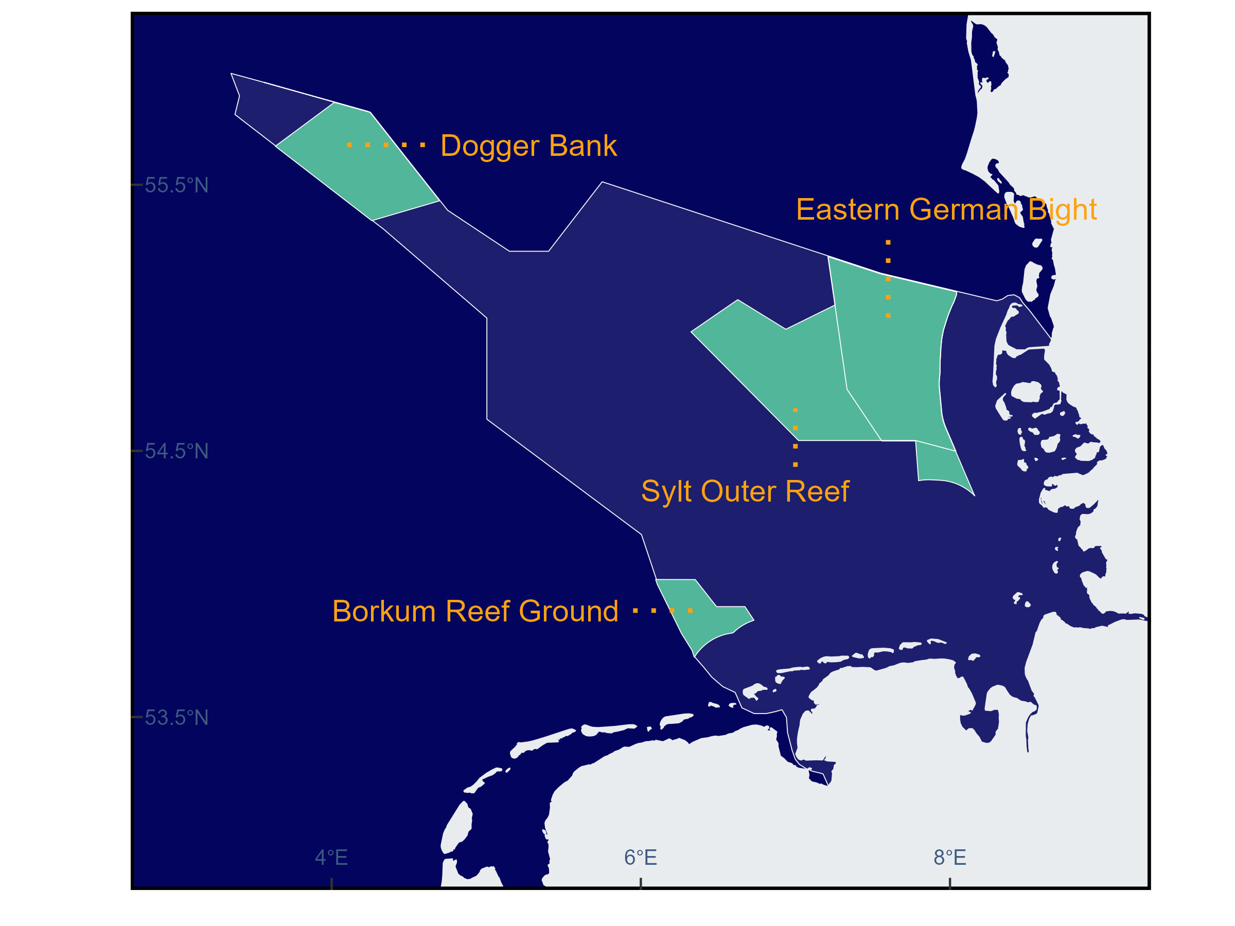

Further reading

In the German North Sea, approximately 46% of the Exclusive Economic Zone (EEZ) is covered by Marine Protected Areas (MPAs) and other nature conservation areas. Specifically, these areas encompass 18,698 km², while the total German North Sea EEZ is 40,999 km² (Biodiversity Europe). However, many activities are allowed in marine protected areas, making effective protection unclear.

Other sources:
- Birds directive - Habitats directive - Natura 2000 - Marine Protected Areas